Constructing Parabolas with Mathematica

There are several ways to draw a parabola using straight lines. If you get a chance, you should try one sometime - it is always satisfying to see the outline of a curve slowly emerging from a collection of straight lines.

One method uses a set-square. As described in A Book of Curves by E.H. Lockwood (page 3):

Draw a fixed line \(AY\) and mark a fixed point \(S\). Place a set square \(UQV\) (right-angled at \(Q\)) with the vertex \(Q\) on \(AY\) and the side \(QU\) passing through \(S\) (Fig. 2). Draw the line \(QV\). When this has been done in a large number of positions, the parabola can be drawn freehand, touching each of the lines so drawn. The curve is said to be the envelope of the variable line \(QV\) (Fig. 1).

I thought it would be fun to reproduce this method in Mathematica. I’ll work through the construction step-by-step. It is a nice introduction to some of Mathematica’s graphics options.

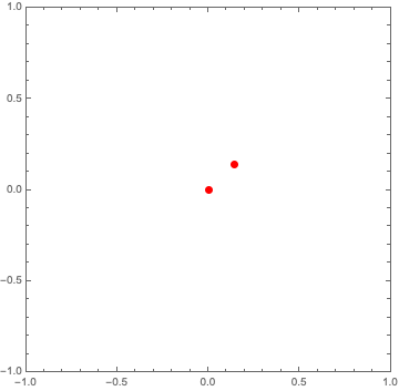
I’ll start with the points \(A\) and \(S\). For simplicity I’ll put \(A\) at the origin, and choose \(S\) to be \( (1/7, 1/7)\).

a = {0, 0};
s = {1/7, 1/7};
Graphics[{
  {PointSize[Large], Red, Point[a]},
  {PointSize[Large], Red, Point[s]}
  },
 PlotRange -> {{-1, 1}, {-1, 1}},
 Frame -> True]

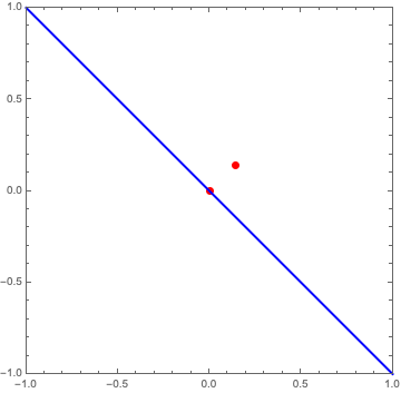
Next comes the line \(AY\). One way to draw this line is to calculate the slope of the line \(AS\), take the negative reciprocal to get the slope of \(AY\), and pass the point \(A\) and the slope to Mathematica’s InfiniteLine. The slope is just \(-S_x/S_y\), which in this specific case comes out to \(-1\).

a = {0, 0};
s = {1/7, 1/7};
slope = -s[[1]]/s[[2]];
Graphics[{
  {PointSize[Large], Red, Point[a]},
  {PointSize[Large], Red, Point[s]},
  {Blue, Thick, InfiniteLine[a, {1, slope}]}
  },
 PlotRange -> {{-1, 1}, {-1, 1}},
 Frame -> True]

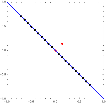
Now we need a number of points along \(AY\) (the blue line above) on which to draw the lines \(QV\). I would like to control both the number of points and the point spacing, so I’ll introduce both of these as variables: numberOfPoints and pointSpacing. Multiplying these together gives a distance travelled along the line \(AY\). Moving in one direction from the origin by this distance, we’ll end up at the point:

$$ (\text{xEnd}, \text{yEnd}) = \left( \frac{d}{\sqrt{1 + m^2}}, \frac{d m}{\sqrt{1 + m^2}} \right) ,$$

where \(d\) is the distance and \(m\) is the slope. Then we can just calculate the step sizes for \(x\) and \(y\), and iterate by this step size until we get to the endpoint. In code form:

distance = numberOfPoints*pointSpacing;
xEnd = distance/Sqrt[1 + slope^2];
xStep = xEnd/numberOfPoints;
yEnd = xEnd*slope;
yStep = yEnd/numberOfPoints;
points = Table[{i*xStep, i*yStep}, {i, 1, numberOfPoints}];

Doing the same for the other direction from the origin, and drawing the points:

a = {0, 0};
s = {1/7, 1/7};
slope = -s[[1]]/s[[2]];
numberOfPoints = 10;
pointSpacing = 0.1;
distance = numberOfPoints*pointSpacing;
xEnd = distance/Sqrt[1 + slope^2];
xStep = xEnd/numberOfPoints;
yEnd = xEnd*slope;
yStep = yEnd/numberOfPoints;
allPoints = Join[
   Table[{i*xStep, i*yStep}, {i, 1, numberOfPoints}],
   Table[{-i*xStep, -i*yStep}, {i, 1, numberOfPoints}]];
Graphics[{
  {PointSize[Large], Red, Point[a]},
  {PointSize[Large], Red, Point[s]},
  {Blue, Thick, InfiniteLine[a, {1, slope}]},
  {PointSize[Large], Point[allPoints]}
  },
 PlotRange -> {{-1, 1}, {-1, 1}},
 Frame -> True]

Note that we end up with a total of 2*numberOfPoints.

Now, at each of these points \(Q\), we need a line that is through the point and perpendicular to the line \(QS\). I’ll construct these lines the same way that I constructed the blue line \(AY\): calculate the slope as the negative reciprocal of the slope of \(QS\), and pass the point \(Q\) and the slope to InfiniteLine. This is probably the most Mathematica-flavored part of the code - I use Map in the shorthand /@ to generate a list of slopes, and MapThread to make the lines.

a = {0, 0};
s = {1/7, 1/7};
slope = -s[[1]]/s[[2]];
numberOfPoints = 10;
pointSpacing = 0.1;
distance = numberOfPoints*pointSpacing;
xEnd = distance/Sqrt[1 + slope^2];
xStep = xEnd/numberOfPoints;
yEnd = xEnd*slope;
yStep = yEnd/numberOfPoints;
allPoints = Join[
   Table[{i*xStep, i*yStep}, {i, 1, numberOfPoints}],
   Table[{-i*xStep, -i*yStep}, {i, 1, numberOfPoints}]];
getSlope[point_] := -(s[[1]] - point[[1]])/(s[[2]] - point[[2]]);
allSlopes = getSlope /@ allPoints;
newline[point_, slope_] := InfiniteLine[point, {1, slope}];
Graphics[{
  {PointSize[Large], Red, Point[a]},
  {PointSize[Large], Red, Point[s]},
  {Blue, Thick, InfiniteLine[a, {1, slope}]},
  {PointSize[Large], Point[allPoints]},
  MapThread[newline, {allPoints, allSlopes}]
  },
 PlotRange -> {{-1, 1}, {-1, 1}},
 Frame -> True]

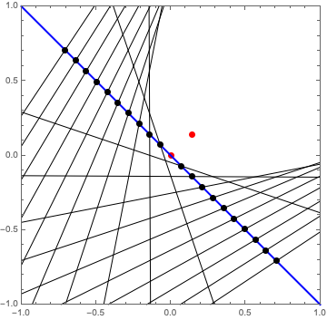
Ok, that is starting to look like a parabola!

To make things easier, I’ll gather everything so far up into a function (and stop explicitly showing the points \(Q\)):

parabola[s_, numberOfPoints_, pointSpacing_] := Module[{},
  a = {0, 0};
  slope = -s[[1]]/s[[2]];
  distance = numberOfPoints*pointSpacing;
  xEnd = distance/Sqrt[1 + slope^2];
  xStep = xEnd/numberOfPoints;
  yEnd = xEnd*slope;
  yStep = yEnd/numberOfPoints;
  allPoints = Join[
    Table[{i*xStep, i*yStep}, {i, 1, numberOfPoints}],
    Table[{-i*xStep, -i*yStep}, {i, 1, numberOfPoints}]];
  getSlope[point_] := -(s[[1]] - point[[1]])/(s[[2]] - point[[2]]);
  allSlopes = getSlope /@ allPoints;
  newline[point_, slope_] := InfiniteLine[point, {1, slope}];
  Graphics[{
    {PointSize[Large], Red, Point[a]},
    {PointSize[Large], Red, Point[s]},
    {Blue, Thick, InfiniteLine[a, {1, slope}]},
    MapThread[newline, {allPoints, allSlopes}]
    },
   PlotRange -> {{-1, 1}, {-1, 1}},
   Frame -> True]]

Then parabola[{1/7, 1/7}, 100, 0.05] gives

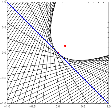
Beautiful!

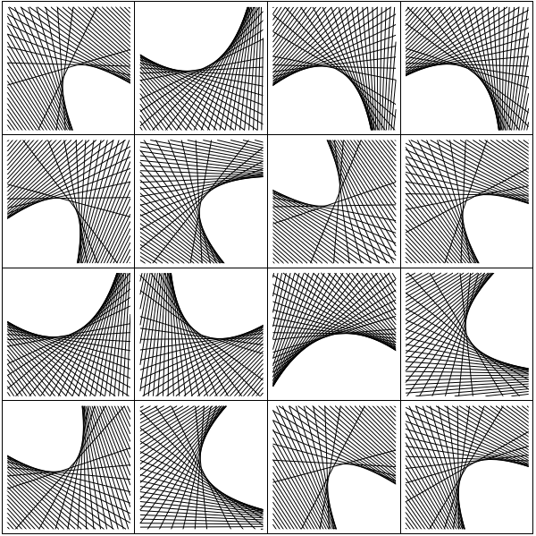
Getting rid of the Frame -> True part and removing all of the graphics except for the final lines lets us generate a bunch of random parabolas this way:

GraphicsGrid[
 Partition[
  Table[
   parabola[{
     RandomChoice[{-1, 1}]/RandomReal[{2, 15}],
     RandomChoice[{-1, 1}]/RandomReal[{2, 15}]}, 50, 0.05],
   {16}], 4],
 Frame -> All]