In chapter 1 of their 2016 book Computer Age Statistical Inference, Bradley Efron and Trevor Hastie use as an example a study of kidney function, comparing results from linear regression and lowess (locally weighted scatterplot smoothing). The purpose of this blog post is to reproduce their results using R.
I will not copy the plots from the book here (for copyright reasons), but you can download a pdf of the book for free from a website created by the authors: https://web.stanford.edu/~hastie/CASI/index.html. I am specifically interested in Figures 1.1 and 1.2, as well as Table 1.1.
Let’s first grab the kidney function data (also kindly provided by the authors on their website):
library(tidyverse)
kidney_data <- read_delim('https://web.stanford.edu/~hastie/CASI_files/DATA/kidney.txt', delim = ' ')

kidney_data
## # A tibble: 157 × 2
##      age   tot
##    <dbl> <dbl>
##  1    18  2.44
##  2    19  3.86
##  3    19 -1.22
##  4    20  2.3
##  5    21  0.98
##  6    21 -0.5
##  7    21  2.74
##  8    22 -0.12
##  9    22 -1.21
## 10    22  0.99
## # ℹ 147 more rows
Just getting the linear regression line is straightforward:
base_plot <- kidney_data %>%
  ggplot(aes(x = age, y = tot)) +
  geom_point(shape = 8, color = 'blue', size = 1) +
  theme_bw() +
  scale_x_continuous(breaks = seq(20, 90, 10)) +
  scale_y_continuous(breaks = seq(-6, 4, 2)) +
  theme(panel.grid.major = element_blank(),
        panel.grid.minor = element_blank())

linear_plot <- base_plot +
  geom_smooth(method = 'lm', color = 'green', se = F)

linear_plot
## `geom_smooth()` using formula = 'y ~ x'
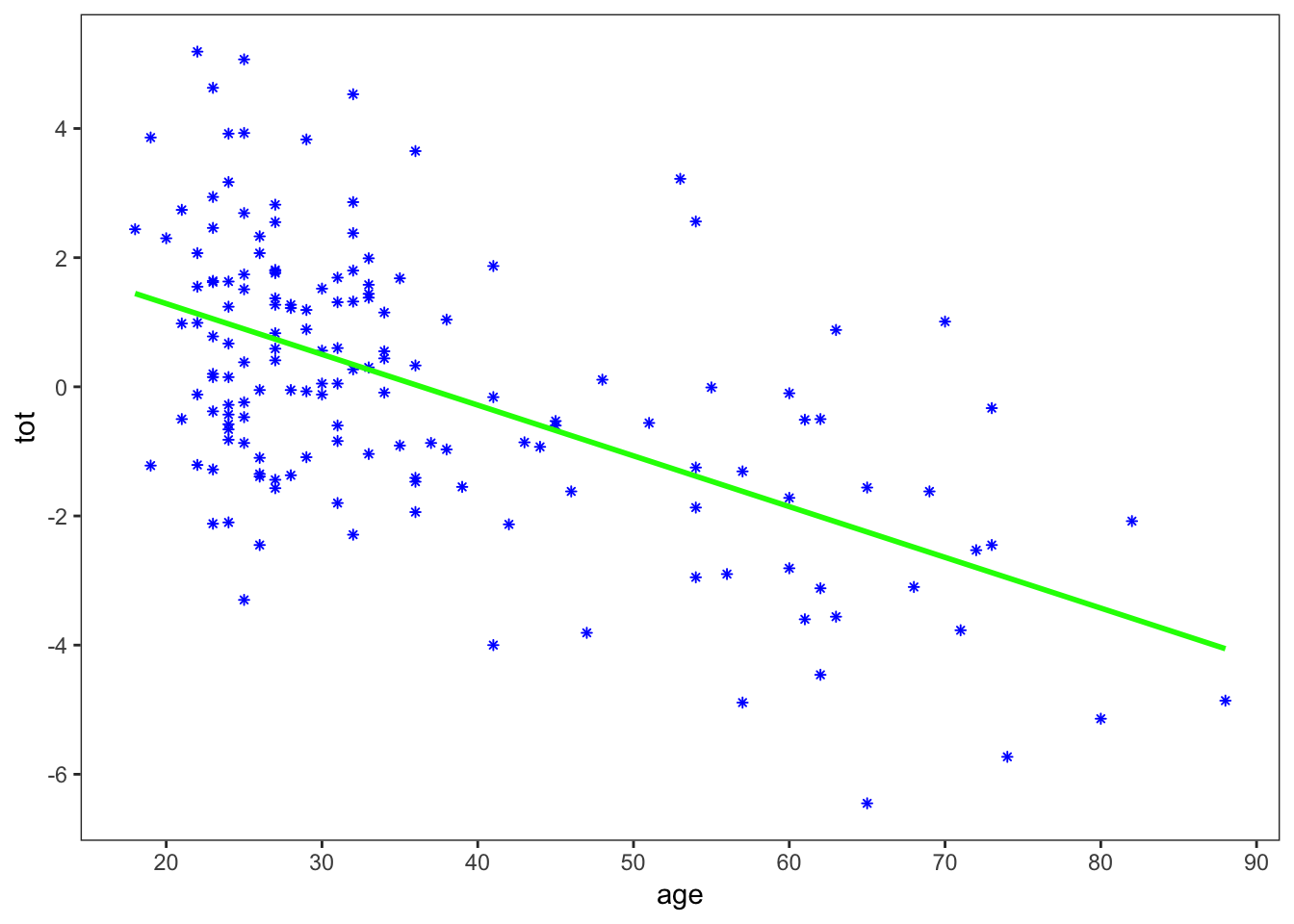
Here I separated out the plot of just the data (base_plot), so that I can use it for both the linear regression plot and the lowess plot. I also went to a little bit of trouble to make the plot in a similar style as Figure 1.1 in the book. It is not an exact copy, but close enough.
I removed the standard error from geom_smooth, since the default is to plot the error as a continuous curve, and Figure 1.1 only shows the error at a few discrete points. Let’s next calculate the standard error at those points:
library(broom)

linear_model <- lm(tot ~ age, data = kidney_data)

error_points <- data.frame(age = seq(20, 80, 10))

linear_error <- augment(linear_model, newdata = error_points, se_fit = TRUE)

linear_error
## # A tibble: 7 × 3
##     age .fitted .se.fit
##   <dbl>   <dbl>   <dbl>
## 1    20   1.29    0.207
## 2    30   0.502   0.155
## 3    40  -0.284   0.147
## 4    50  -1.07    0.189
## 5    60  -1.86    0.258
## 6    70  -2.64    0.337
## 7    80  -3.43    0.420
Now add the error bars to the linear plot:
linear_plot +
  geom_segment(data = linear_error,
               aes(x = age, xend = age,
                   y = .fitted - 2*.se.fit, yend = .fitted + 2*.se.fit))
## `geom_smooth()` using formula = 'y ~ x'
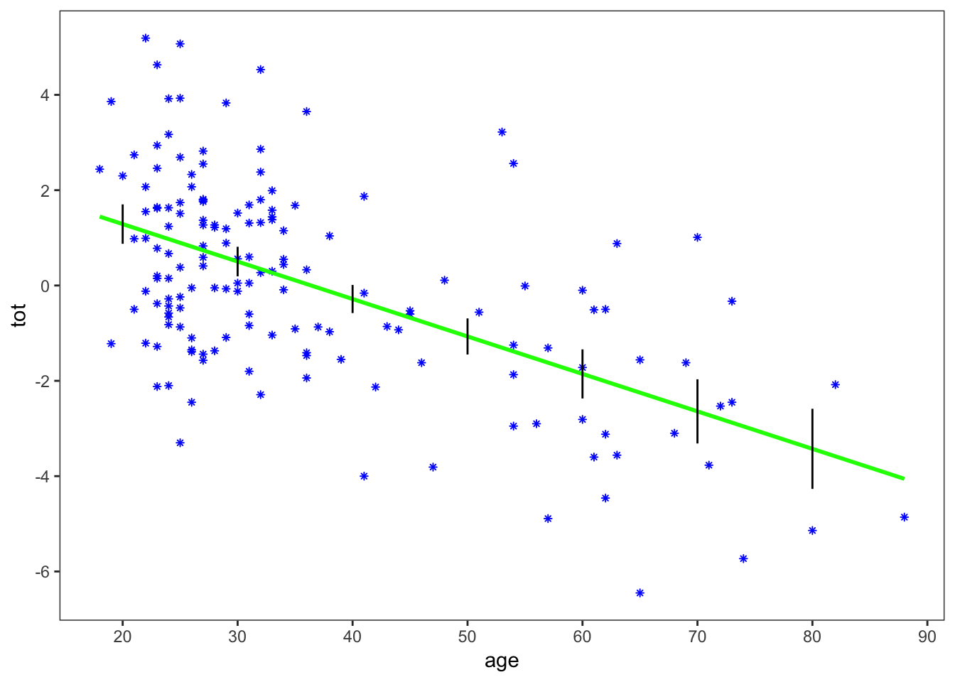
The plot shows \(\pm2\) standard errors at each of the 7 selected age values. This is a good replication of Figure 1.1.
For Figure 1.2, the authors use the lowess algorithm in R, which stands for ‘locally weighted scatterplot smoothing.’ There is an updated version in R named loess, and I assume there is some mapping between the two, but it is not immediately obvious, so I will stick with lowess.
Again, obtaining just the lowess fit is fairly straightforward, except for the fact that geom_smooth uses loess and not lowess, so we have to calculate the fit ‘by hand’ (i.e. outside of ggplot) and then add it to the plot:
lowess_model <- lowess(kidney_data$age, kidney_data$tot, 1/3) %>%
  as_tibble()

lowess_plot <- base_plot +
  geom_line(data = lowess_model, aes(x = x, y = y), color = 'green')

lowess_plot
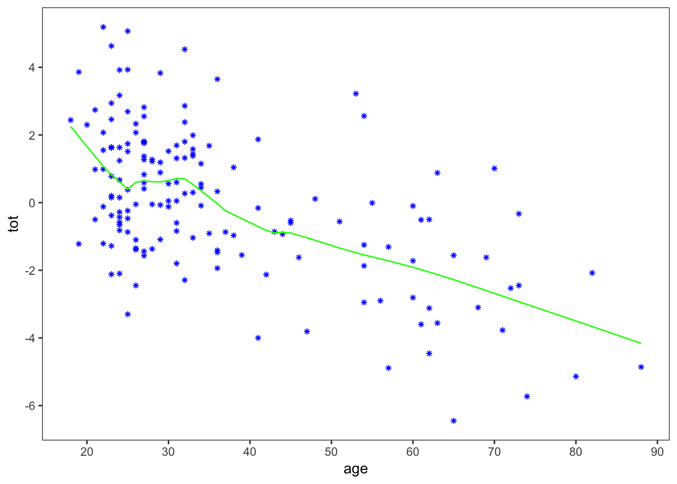
The ‘1/3’ in lowess is a parameter governing the smoothness of the fit. Now, to get the standard errors for the lowess fit, the authors use the bootstrap. This is not the place for a full-fledged introduction to the bootstrap, but in brief it is a way of approximating the standard error by repeatedly sampling with replacement from the original data. There are many ways to run a bootstrap sample in R: here I’ll uses bootstraps from the rsample package:
library(rsample)
## Registered S3 method overwritten by 'future':
##   method               from
##   all.equal.connection parallelly
bootstrap_samples <- bootstraps(kidney_data, times = 25)

bootstrap_samples
## # Bootstrap sampling
## # A tibble: 25 × 2
##    splits           id
##    <list>           <chr>
##  1 <split [157/60]> Bootstrap01
##  2 <split [157/50]> Bootstrap02
##  3 <split [157/55]> Bootstrap03
##  4 <split [157/56]> Bootstrap04
##  5 <split [157/56]> Bootstrap05
##  6 <split [157/55]> Bootstrap06
##  7 <split [157/59]> Bootstrap07
##  8 <split [157/63]> Bootstrap08
##  9 <split [157/61]> Bootstrap09
## 10 <split [157/54]> Bootstrap10
## # ℹ 15 more rows
Each sample (split) contains an “analysis” data set that is the same length as the original kidney_data, and an “assessement”" data set containing all the original data points that did not get included in the bootstrap sampling with replacement. Now, for each of these bootstrap samples, we want to apply a lowess fit, so let’s write a function that does that and then map it over the bootstraps:
lowess_fit <- function(split){
  lowess(analysis(split)$age, analysis(split)$tot, 1/3)
}

bootstrap_samples %>%
  mutate(lowess_points = map(splits, lowess_fit)) %>%
  select(id, lowess_points) %>%
  mutate_if(is.list, map, as_data_frame) %>%
  unnest()
## # A tibble: 3,925 × 3
##    id              x     y
##    <chr>       <dbl> <dbl>
##  1 Bootstrap01    18  2.17
##  2 Bootstrap01    18  2.17
##  3 Bootstrap01    20  1.66
##  4 Bootstrap01    21  1.40
##  5 Bootstrap01    21  1.40
##  6 Bootstrap01    22  1.11
##  7 Bootstrap01    22  1.11
##  8 Bootstrap01    22  1.11
##  9 Bootstrap01    22  1.11
## 10 Bootstrap01    22  1.11
## # ℹ 3,915 more rows
Let’s plot these 25 bootstrapped replications of the lowess fit, along with the original data. I’ll add a distinct because I don’t care about multiple identical values for plotting purposes:
lowess_25 <- bootstrap_samples %>%
  mutate(lowess_points = map(splits, lowess_fit)) %>%
  select(id, lowess_points) %>%
  mutate_if(is.list, map, as_data_frame) %>%
  unnest() %>%
  distinct()
base_plot +
  geom_line(data = lowess_25, aes(x = x, y = y, color = id),
            alpha = 0.5) +
  theme(legend.position = 'none')
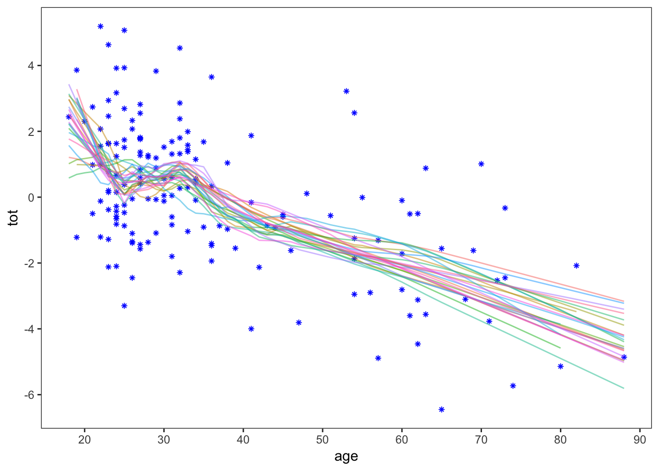
This gives a rough idea of the standard error of the lowess fit. Now, as did Efron and Hastie, we’ll take 250 bootstrap samples and calculate the standard error. First, we need a function that will give the lowess fit at the same 7 points where we calculated the standard error of the linear model. Since lowess outputs a series of \(x\) and \(y\) values, I’ll just use linear interpolation between these values:
lowess_predict <- function(fit){
  approx(fit %>% as_tibble() %>% distinct(), xout = seq(20, 80, 10), rule = 2)
}
(rule = 2 allows extrapolation outside the input data range, which is necessary since the bootstrap sample won’t always contain the extrema of the original data set.)
Now, for the full 250 replications. I’ll break this into 2 steps so it is more clear what is going on.
step_1 <- bootstraps(kidney_data, times = 250) %>%
  mutate(lowess_points = map(splits, lowess_fit)) %>%
  mutate(prediction = map(lowess_points, lowess_predict)) %>%
  select(id, prediction) %>%
  mutate_if(is.list, map, as_data_frame) %>%
  unnest()
step_1
## # A tibble: 1,750 × 3
##    id               x       y
##    <chr>        <dbl>   <dbl>
##  1 Bootstrap001    20  2.00
##  2 Bootstrap001    30  0.256
##  3 Bootstrap001    40 -0.0372
##  4 Bootstrap001    50 -1.14
##  5 Bootstrap001    60 -1.69
##  6 Bootstrap001    70 -2.26
##  7 Bootstrap001    80 -2.91
##  8 Bootstrap002    20  1.54
##  9 Bootstrap002    30  0.570
## 10 Bootstrap002    40 -0.841
## # ℹ 1,740 more rows
step_2 <- step_1 %>%
  group_by(x) %>%
  summarise(mean = round(mean(y), 2),
            sd = round(sd(y), 2))

step_2
## # A tibble: 7 × 3
##       x  mean    sd
##   <dbl> <dbl> <dbl>
## 1    20  1.61  0.65
## 2    30  0.64  0.25
## 3    40 -0.61  0.36
## 4    50 -1.27  0.34
## 5    60 -1.92  0.37
## 6    70 -2.64  0.5
## 7    80 -3.36  0.73
These mean and standard deviation values match fairly well with the values given in Table 1.1 of Computer Age Statistical Inference, with the caveat that the authors only did 250 bootstrap replications, and we only did 250 bootstrap replications, so we shouldn’t expect exact agreement.
Let’s add the bootstrap standard errors to the plot of the lowess fit:
lowess_plot +
  geom_segment(data = step_2,
               aes(x = x, xend = x,
                   y = mean - 2*sd, yend = mean + 2*sd))
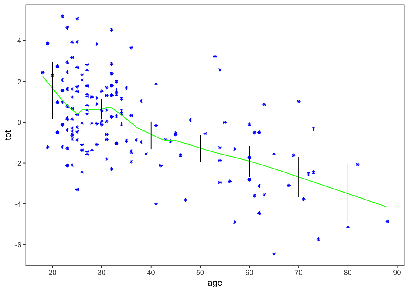
This provides a good replication of Figure 1.2 in the book.
As always, I am sure that there are other ways to accomplish the same result in R, likely including ones that are more concise and clear. If you have a nice approach (or if you find a mistake in what I’ve done), please send me an email and let me know!