Consider a multinomial distribution with \(c\) categories and associated probabilities \(\pi_i\), where \(i = 1,...,c\). It is often useful to be able to estimate the ratio of the probabilities of two of the categories from observed data. Without loss of generality, let these two categories be 1 and 2, so that the desired ratio is \(\phi = \pi_1/\pi_2\).
Putting a Dirichlet prior on the multinomial priors \(\pi_i\) results in a Dirichlet posterior, since the Dirichlet distribution is a conjugate prior for the multinomial likelihood. With the Dirichlet prior as
$$
\text{Dirichlet}(a_1, …, a_c) = \frac{\Gamma(a_1 + \dots + a_c)}{\Gamma(a_1) \cdots \Gamma(a_c)}\pi_1^{a_1 - 1}\cdots \pi_c^{a_c -1},
$$
the posterior distribution is \(\text{Dirichlet}(a_1 + n_1, \dots , a_c + n_c)\), where \(n_i\) is the number of observations in category \(i\). The posterior mean of the parameter \(\pi_i\) is then
$$
\frac{n_i + a_i}{n + K}
$$
where \(K = \sum_i a_i\).
A first guess for a point estimate of \(\phi\) might be to take the ratio of the posterior means of \(\pi_1\) and \(\pi_2\), giving
$$
\frac{n_1 + a_1}{n_2 + a_2}.
$$
But there is no reason that, in general, the ratio of the posterior means should equal the posterior mean of the ratio. Before going further and doing things correctly, let’s note a couple things about this point estimate. It does not depend on the observations in other categories, or even on the total number of categories \(c\). This makes sense, as \(\phi\) is logically independent of what is going on in the other categories. Also, this point estimate is similar to what you get by using maximum likelihood inference. In that case, the maximum likelihood estimate of \(\pi_i\) is \(\hat{\pi}_i = n_i/n\), the sample proportion in that category. And since maximum likelihood inference enjoys an invariance property, it is the case that the maximum likelihood estimate of the ratio is the ratio of the maximum likelihood estimates:
$$
\hat{\phi} = \frac{\hat{\pi}_1}{\hat{\pi}_2} = \frac{n_1}{n_2}.
$$
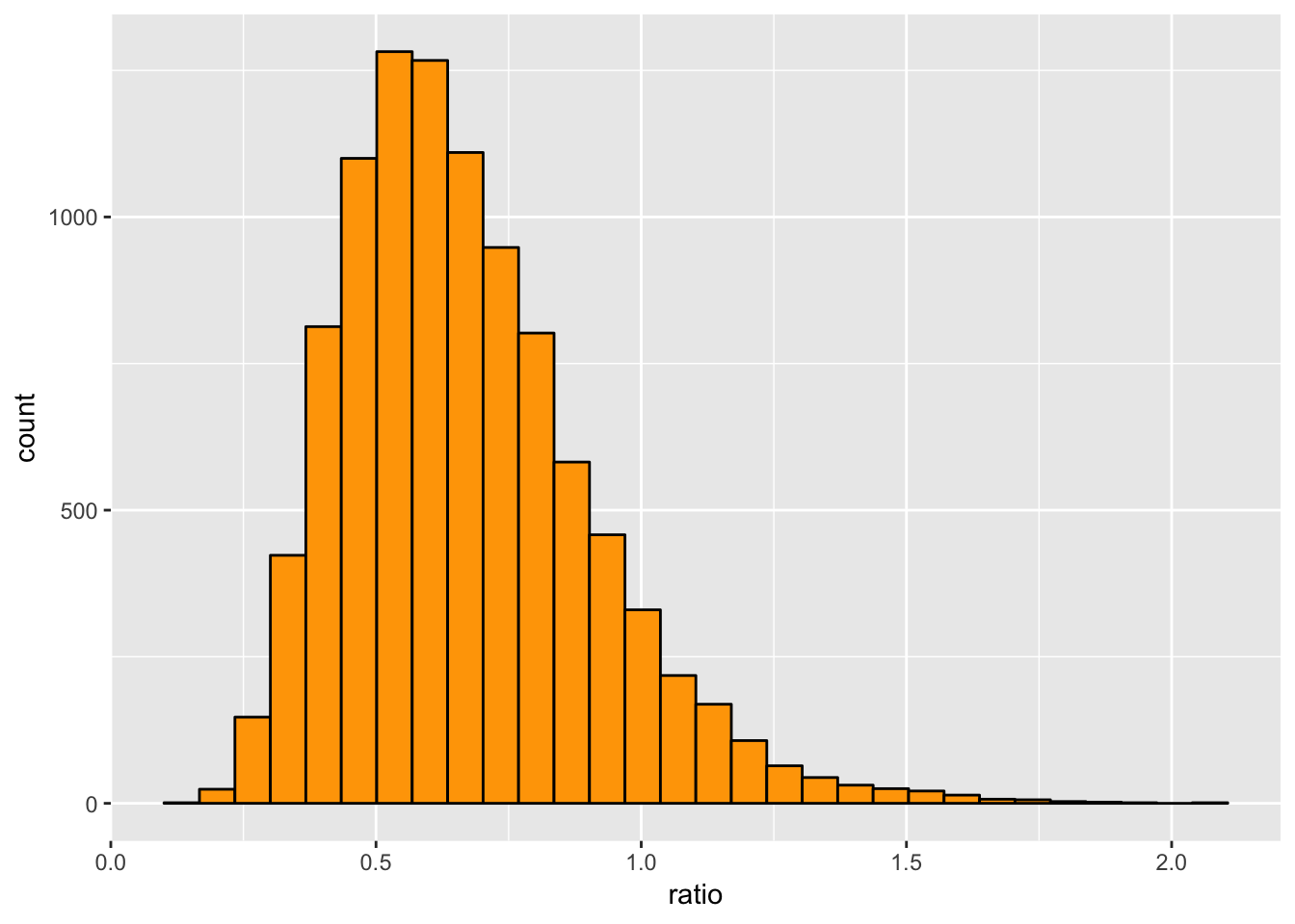
Returning to the Bayesian estimate, let’s do things the easy way and simulate to get the answer. Take the number of categories \(c = 3\) and a prior with \(a_1 = 4\), \(a_2 = 2\), and \(a_3 = 2\). Assume you observe \(n_1 = 10\), \(n_2 = 20\), and \(n_3 = 30\). Then, using 10000 draws from the posterior, the distribution of \(\phi = \pi_1/\pi_2\) looks like
library(tidyverse)
library(MCMCpack)
rdirichlet(10000, c(4 + 10, 2 + 20, 2 + 30)) %>%
  as_tibble() %>%
  mutate(ratio = V1/V2) %>%
  ggplot(aes(x = ratio)) +
  geom_histogram(color = "black", fill = "orange")
 We can calculate the posterior mean of the ratio and compare to the ratio of posterior means:
rdirichlet(10000, c(4 + 10, 2 + 20, 2 + 30)) %>%
  as_tibble() %>%
  mutate(ratio = V1/V2) %>%
  summarise_all(funs(mean)) %>%
  mutate(ratio_of_means = V1/V2) %>%
  mutate_all(funs(round(.,3))) %>%
  knitr::kable(align = rep('c', 5))
| V1 | V2 | V3 | ratio | ratio_of_means |
|---|---|---|---|---|
| 0.206 | 0.324 | 0.47 | 0.668 | 0.638 |
I haven’t bothered renaming the columns, so \(V1 = \pi_1\) and so on. With \(K = 4 + 2 + 2 = 8\), \(n = 10 + 20 + 30 = 60\) (and rounding to three decimal places), the theoretical values are \(E[V1] = (10 + 4)/(60 + 8) = 0.206\), \(E[V2] = (20 + 2)/(60 + 8) = 0.324\), \(E[V3] = (30 + 2)/(60 + 8) = 0.471\), and the ratio of posterior means is \((10 + 4)/(20 + 2) = 0.636\). The simulation using 10000 draws is more than enough to show that the posterior mean of the ratio is definitely not the same as the ratio of the posterior means.
We can verify that the posterior mean of the ratio does not depend on the observations in other categories or the total number of categories. First, changing \(n_3\) from 30 to 20:
rdirichlet(10000, c(4 + 10, 2 + 20, 2 + 20)) %>%
  as_tibble() %>%
  mutate(ratio = V1/V2) %>%
  summarise_all(funs(mean)) %>%
  mutate(ratio_of_means = V1/V2) %>%
  mutate_all(funs(round(.,3))) %>%
  knitr::kable(align = rep('c', 5))
| V1 | V2 | V3 | ratio | ratio_of_means |
|---|---|---|---|---|
| 0.241 | 0.379 | 0.38 | 0.664 | 0.634 |
Next, adding a category (going from \(c = 3\) to \(c = 4\)):
rdirichlet(10000, c(4 + 10, 2 + 20, 2 + 20, 3 + 30)) %>%
  as_tibble() %>%
  mutate(ratio = V1/V2) %>%
  summarise_all(funs(mean)) %>%
  mutate(ratio_of_means = V1/V2) %>%
  mutate_all(funs(round(.,3))) %>%
  knitr::kable(align = rep('c', 6))
| V1 | V2 | V3 | V4 | ratio | ratio_of_means |
|---|---|---|---|---|---|
| 0.153 | 0.242 | 0.242 | 0.363 | 0.663 | 0.633 |
This is nice, but what is the theoretical value of the posterior mean of the ratio? It is
$$
E[\phi] = \frac{n_1 + a_1}{n_2 + a_2 -1},
$$
which in our example works out to \((4 + 10)/(2 + 20 - 1) = 0.667\) (rounded to three decimal places). This is close to the ratio of the posterior means, but a little higher, and agrees with the simulated values above. The proof of this formula is a nice calculus exercise, which I might write up as a future blog post. In general, the posterior mean of the ratio \(\pi_i/\pi_j\) is
$$
E\left[\frac{\pi_i}{\pi_j}\right] = \frac{n_i + a_i}{n_j + a_j - 1}.
$$
I became interested in this problem while reading Categorical Data Analysis by Agresti (3rd edition). Part of Problem 38 in Chapter 1 reads as follows: “For a Dirichlet prior, show that using the Bayes estimates of \(\pi_i\) and \(\pi_j\) to estimate \(\pi_i/\pi_j\) uses also the counts in other categories.” Based upon the above simulations (and the promised calculation of the expected value of the ratio), I believe that this problem is incorrect as stated. (One might object that the posterior means might stay the same upon changing the number of categories, but the posterior distribution changes. The same exercise the produces the posterior mean gives the posterior distribution along the way and shows that the distribution does not depend on the number of categories or the counts in other categories.)