Bayesian Decision Boundaries

I started reading The Elements of Statistical Learning by Hastie, Tibshirani, and Friedman, and was curious about how to reproduce Figure 2.5. (The book is made available as a free and legal pdf here.)

So I figured out how to produce similar figures using Mathematica. I assume that this is also fairly straightforward to do in R, but I don’t yet know enough R.

The authors explain the sampling method on pages 16 and 17. First, select 10 vectors from a multivariate Gaussian centered on the unit x-vector, then select another 10 from a Gaussian centered on the unit y-vector.

Here is the Mathematica code to do this:

blue = RandomReal[MultinormalDistribution[{1,0}, IdentityMatrix[2]], 10];
orange = RandomReal[MultinormalDistribution[{0,1}, IdentityMatrix[2]], 10];

Now, for each class (blue and orange), pick 100 points by first picking one of the 10 vectors in that class at random, then using that vector as the center of another distribution from which a point is selected. I call the two classes of 100 points set 1 and set 2:

set1 = Table[
   RandomReal[
    MultinormalDistribution[Evaluate[RandomChoice[blue]], IdentityMatrix[2]/5]], 100];
set2 = Table[
   RandomReal[
    MultinormalDistribution[Evaluate[RandomChoice[orange]], IdentityMatrix[2]/5]], 100];

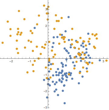
We can now plot the resulting 200 points:

listplot = 
  ListPlot[{set1, set2}, PlotRange -> All, AspectRatio -> 1, 
  PlotStyle -> {PointSize[0.02]}];

Result:

Now, for the decision boundary, just set the probability that a point comes from set 1 equal to the probability that a point comes from set 2. This means setting a sum over 10 Gaussians equal to another sum over 10 Gaussians, so it takes some time to evaulate a grid of points to make a contour plot. You can choose a lower number of PlotPoints to make this faster, but this makes the curve more jagged.

Here is the Mathematica code, followed by the result of overlaying both plots:

contourplot = ContourPlot[
   Sum[PDF[
      MultinormalDistribution[orange[[ii]], IdentityMatrix[2]/5], {xx, yy}], {ii, 1, 10}] ==
    Sum[PDF[
      MultinormalDistribution[blue[[jj]], IdentityMatrix[2]/5], {xx, yy}], {jj, 1, 10}],
   {xx, -5, 5}, {yy, -5, 5}, PlotPoints -> 35, Axes -> True, 
   ContourStyle -> {Red, AbsoluteThickness[2]}];
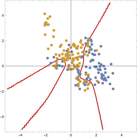
Show[listplot, contourplot]

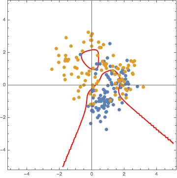
Ok, so the cluster around \(y = 1.5\) is not filled out, but we only sampled a total of 200 points, so that’s alright.

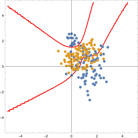
Now, this doesn’t look exactly like Figure 2.5 in Elements of Statistical Learning, but of course the specific form of the plot depends heavily on the initial 20 random vectors. Here are some sample results after rerunning the code:

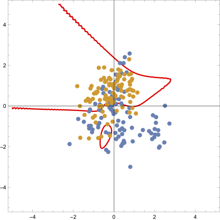
I put the code on my github in the form of a loop to generate and save 10 of the above plots.