Here is an interesting problem having to do with dice and probability.
Take a normal, fair die. Instead of labeling the faces with the numbers 1 to 6, label two of the faces with the number 1, then the remaining four faces with the numbers 2 to 5. So instead of
\[ \text{sides} = \{1, 2, 3, 4, 5, 6\}, \]
we have
\[ \text{sides} = \{1, 1, 2, 3, 4, 5\}. \]
Given this new die, roll it repeatedly and record the results of each roll. What is the probability that you will roll 6 ones before you roll 6 twos?
For a single roll, the probability of rolling a one is \(1/3\), and the probability of rolling a two is \(1/6\), so the probability of rolling 6 ones before 6 twos should be greater than \(0.5\).
Let’s start with a simpler problem first. What is the probability of rolling a single one before you roll a two? This should also be greater than \(0.5\). To abstract the problem a bit, I’ll let \(p_1\) stand for the probability of rolling a one and \(p_2\) stand for the probability of rolling a two.
The probability of rolling a one on the first roll is \(p_1\). The probability of getting the first one on the second roll (without getting a two on the first roll) is \(p_1(1 - p_1 - p_2)\), since the second roll has to be a one, and the first roll cannot be a one or a two. In general, the probability of rolling a one for the first time on the \(k\)th roll with no previous twos is \(p_1(1-p_1-p_2)^{k-1}\). Summing over all values of \(k\), we get
\[\text{probability(1 before 2)} = \sum_{k = 1}^\infty p_1(1-p_1 - p_2)^{k-1}. \]
This is a geometric series, and is easily summed to give
\[\text{probability(1 before 2)} = \frac{p_1}{p_1 + p_2}. \]
For our values of \(p_1\) and \(p_2\), this comes out to \(2/3\).
What about rolling two ones before you roll two twos? I’ll jump straight to the generic case of this happening on the \(k\)th roll, and split into 2 cases: either a single 2 was rolled somewhere in the previous \(k-1\) rolls, or no twos were rolled. If no twos were rolled before, we get the term \(p_1^2 (1 - p_1 - p_2)^{k-2} (k - 1)\). Here the factor of \(k-1\) accounts for the \(k - 1\) possible locations of the first 1 roll. If a single 2 was rolled before, we get \(p_1^2 p_2 (1 - p_2 - p_2)^{k-3} (k - 1)(k - 2)\), accounted for the \(k - 1\) possible locations of the 1 roll, and \(k - 2\) possible locations of the 2 roll. Summing over all possible \(k\) values:
\[\text{probability(two 1s before two 2s)} = \sum_{k = 2}^\infty p_1^2 (1 - p_1 - p_2)^{k-2} (k - 1) + \sum_{k = 3}^\infty p_1^2 p_2 (1 - p_2 - p_2)^{k-3} (k - 1)(k - 2) . \]
Doing the sums:
\[\text{probability(two 1s before two 2s)} = \frac{p_1^2 (p_1 + 3 p_2) }{(p_1 + p_2)^3}. \]
For our values of \(p_1\) and \(p_2\), this comes out to \(20/27 \approx 0.7407 \). Note that this is higher than the probability of rolling a single 1 before a single 2.
It would be possible to continue like this until we get up to the case of six 1s before six 2s. But it is not too hard to do the general case: \(N\) 1s before \(N\) 2s. The probability that this happens on the \(k\)th roll can be split into \(j\) cases, where \(j\) goes from \(0\) to \(N - 1\), and in the \(j\)th case \(j\) 2s have been rolled in the previous \(k - 1\) rolls. So we get a sum over terms that look like
\[ p_1^N p_2^j (1 - p_1 - p_2)^{k - N -j} {{k-1}\choose{N-1}}{{k-N}\choose{j}} .\]
The factor of \({{k-1}\choose{N-1}}\) accounts for the ways that the \(N-1\) previous 1s can show up in the \(k-1\) previous rolls, and the factor of \( {{k-N}\choose{j}}\) accounts for the ways that the \(j\) previous 2s can show up in the remaining \(k-N\) previous rolls.
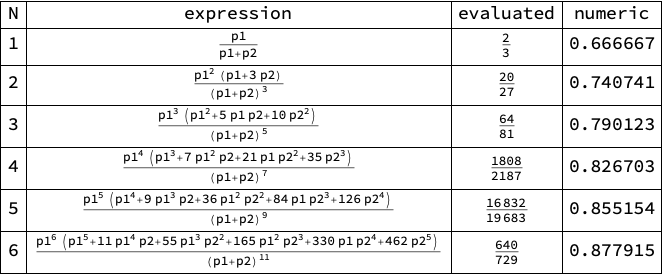
Mathematica can do the sums:
results = Table[{n, x = Simplify[
      Sum[
       Total[
        Table[
         p1^n p2^j (1 - p1 - p2)^(k - n - j)
           Binomial[k - 1, n - 1] Binomial[k - n, j] Boole[k - n - j >= 0],
           {j, 0, n - 1}]],
       {k, 0, \[Infinity]}]],
       p = x /. {p1 -> 1/3, p2 -> 1/6}, N[p]},
   {n, 1, 6}];
Grid[Prepend[
    results, {"N", "expression", "evaluated", "numeric"}],
  Frame -> All]
I checked these theoretical results by simulating the problem in R. Here is a function that performs one iteration or trial of the problem:
iteration <- function(total){
  ones <- 0
  twos <- 0
  while (ones < total && twos < total) {
    roll <- sample(c(1, 1, 2, 3, 4, 5), size = 1)
    if (roll == 2) { twos <- twos + 1 }
    if (roll == 1) { ones <- ones + 1 }
  }
  winner <- if (ones == total) { 1 } else { 0 }
  return(winner)
}
Running sum(replicate(10000, iteration(1)))/10000 gives 0.67, fairly close to the theoretical result for \(N = 1\). Here is a table of the theoretical and simulated results for \(N\) going from 1 to 6, with 100,000 trials for each value of \(N\):
| N | theory | simulation |
|---|---|---|
| 1 | 0.66667 | 0.66701 |
| 2 | 0.74074 | 0.73888 |
| 3 | 0.79012 | 0.79064 |
| 4 | 0.82670 | 0.82635 |
| 5 | 0.85515 | 0.85531 |
| 6 | 0.87792 | 0.87594 |
There are several possibilities for further exploration of this problem. First, the method I used to calculated the probabilities does not scale well as \(N\) increases. The time it takes Mathematica to calculate higher values of \(N\) seems to go up exponentially. There is probably a simpler way to get the terms without doing the sums over \(k\), likely by using generating functions.
An alternate way to calculate the probabilities might also give insight into the limit as \(N \to \infty \). The first few are increasing (this can probably be proved in general), and since they are bounded above by \(1\), there should be a finite limit as \(N \to \infty \). What is this limit?
Finally, the simulation code I wrote in R is not very efficient. What is a better way to do simulations like this as \(N\) increases? (As \(N\) increases, the probability that several of the trials will run for a very long time increases as well.) Is there a way to write the simulation code that avoids the possibility of very-long-running trials?