In my last post, I discussed the geometric mean and how it relates to the more familiar arithmetic mean. I mentioned that the geometric mean is often useful for estimation in physics.
Lawrence Weinstein, in his book Guesstimation 2.0, gives a mental algorithm for approximating the geometric mean. Given two numbers in scientific notation \[ a \times 10^x \quad \text{and}\quad b \times 10^y, \] where the coefficients \(a\) and \(b\) are both between 1 and 9.99, first take the arithmetic mean of \(a\) and \(b\). This is the coefficient of your answer. Then take the arithmetic mean of \(x\) and \(y\), but if \(x + y\) is odd, round the exponent down to the nearest integer and multiply your result by 3. For example, if your two numbers are \[ 3 \times 10^6 \quad \text{and} \quad 5 \times 10^8, \] then the approximation for the geometric mean is \(4 \times 10^7\). The actual value is \(3.873 \times 10^7\), so this is not bad for estimation purposes. For another example, where you have to multiply by 3, take \[ 3 \times 10^6 \quad \text{and} \quad 5 \times 10^9. \] The approximation here gives \(4\cdot 3 \times 10^7 = 1.2 \times 10^8\) (remember to keep the coefficient between 1 and 9.99), and the actual value is \(1.225\times 10^8\) so again not too bad.
How good is this approximation in general? Where does it perform the worst?
First, look at the “round down and multiply by 3” rule. If the exponents sum to an even number, there is no approximation. If they sum to an odd number, we are using \(3\) to approximate \(\sqrt{10} = 3.16228\). So this will undershoot the correct answer. The absolute error will grow without bound as we move to larger exponents, but the relative error is \[ \frac{\sqrt{10} - 3}{\sqrt{10}} = 0.05132, \] or about \(5.1\%\).
Second, look at the other approximation. For the coefficients, we are approximating the geometric mean by the arithmetic mean. This overshoots the correct answer. Recall from my last post that the geometric mean is always less than or equal to the arithmetic mean, which is the famous AM-GM inequality: \[ \sqrt{a b} \leq \frac{a + b}{2}. \] Equality only holds (there is no approximation) if \(a = b\). How bad can this approximation get? Recall that the coefficients \(a\) and \(b\) are restricted to be between \(1\) and \(9.99\) (technically they have to be in the interval \([1,10)\), but using \([1,9.99]\) is good enough for estimation purposes). If we look at the difference \[ f(a, b) = \frac{a+b}{2} - \sqrt{a b}, \] and take the second derivative with respect to \(a\), we get \[ \frac{ \partial^2 f(a,b)}{\partial a^2} = \frac{b^2}{4 (a b)^{3/2}}.\] (Since \(f(a,b)\) is symmetric in \(a\) and \(b\), it doesn’t matter if we take the derivative with respect to \(a\) or \(b\).) The second derivative is always positive, so \(f(a,b)\) does not have a global maximum. If we restrict \(a\) and \(b\) to \([1,9.99]\), \(f(a,b)\) is maximized when \(a = 1\) and \(b = 9.99\), with a maximum of \(2.3343\) (since there is no global maximum, the maximum must be on the boundaries of the interval). The actual value of the geometric mean here is \(\sqrt{9.99} = 3.1607\), so we have a relative error of \(2.3343/3.1607 = 0.7385\), or about \(74\%\).
Because the two approximations act in opposite directions (one overshoots and the other undershoots), the maximum relative error of the mental approximation to the geometric mean is \(74\%\). This is actually not too bad, especially since we are only interested in estimating to the nearest power of 10. For example, the relative error is maximized if we take \[ 1 \times 10^7 \quad \text{and} \quad 9.99 \times 10^{11}. \] The approximation gives \(5.495 \times 10^9\) and the actual geometric mean is \(3.1607 \times 10^9\).
Here is a plot for the absolute value of the relative error, fixing the first number at \(9.99 = 9.99 \times 10^0\) and allowing the second number to vary up to \(1\times 10^8\):
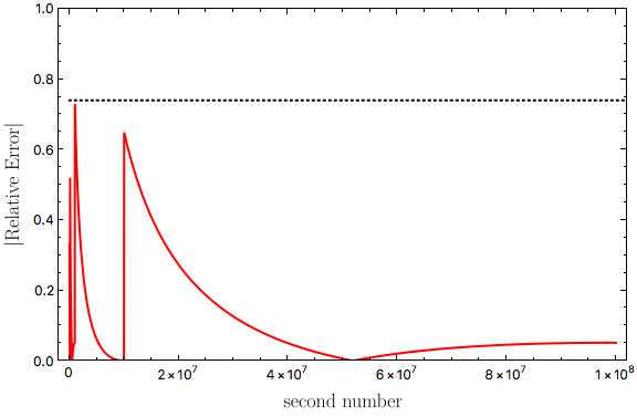
The horizontal dotted line is at a relative error of \(0.74\). I produced this plot using Mathematica, and my implementation of the approximation was
approx[a_?NumericQ, b_?NumericQ] :=
 Block[{aexp, bexp, acoef, bcoef},
  aexp = MantissaExponent[a][[2]] - 1;
  bexp = MantissaExponent[b][[2]] - 1;
  acoef = MantissaExponent[a][[1]]*10.;
  bcoef = MantissaExponent[b][[1]]*10.;
  If[
   EvenQ[aexp + bexp],
   Mean[{acoef, bcoef}] 10^Mean[{aexp, bexp}],
   3*Mean[{acoef, bcoef}] 10^Floor[Mean[{aexp, bexp}]]
   ]
  ]
Interested in finding out how physics, applied math, and data science can help your project or organization? Contact me at landonlehman@gmail.com for a free 15 minute consultation.